Generating and Saving Random Effect Estimates in SPSS
(Versions Earlier than 25)

Note: As of version 25, SPSS now includes an option to print the random effect estimates to the output window (by including the SOLUTION option on the /RANDOM subcommand). The Output Management System (OMS) can then be used to save these estimates to a data file. Please see our instructions on how to use this new approach. The current page indicates how random effect estimates can be generated in prior versions of SPSS.

Like SAS, Stata, R, and many other statistical software programs, SPSS provides the ability to fit multilevel models (also known as hierarchical linear models, mixed-effects models, random effects models, and variance component models). Unlike many other programs, however, one feature that SPSS did not offer prior to Version 25 is the option to output estimates of the random effects. Obtaining estimates of the random effects can be useful for a variety of purposes, for instance to conduct model diagnostics. Plots involving these estimates can help to evaluate whether the random effects are plausibly normally distributed, whether there are extreme values, and whether predictors may have omitted nonlinear effects. Sometimes it is also of interest to rank cases by the estimated values of the random effects, or to use the random effect estimates for the purpose of plotting individual trajectories (particularly in the presence of covariates). Thus, we would like to be able to obtain these estimates from SPSS, just as we can with other software options for fitting multilevel models.

There is more than one way to coax SPSS into providing us with the random effect estimates. In past offerings of our multilevel modeling workshop, we provided syntax that back-solved for the random effect estimates using the model-implied predicted outcome values (which SPSS will nicely output). That approach, however, is somewhat opaque, cumbersome, and limited in its applicability, so here we present an alternative approach, namely, implementing the proper equations to directly estimate the random effects based on the model estimates and observed data. The syntax file that we've developed is designed to produce random effect estimates (empirical Bayes' estimates, to be specific) for models of the following form:

• • Two-level data (including growth models)
  • A multilevel linear model (i.e., a continuous outcome variable; not a multilevel generalized linear model)
  • Independent and homoscedastic level 1 residuals (the default assumption of SPSS), although this could be relaxed with modest modifications to the syntax

For any given analysis, minor changes to the syntax will be required to reflect the data and model at hand, for instance indicating variable names and inputting some model estimates, as described below via an example application.

Downloads

You may wish to right-click these links and choose "Save As" to preserve formatting.

• Syntax File for Computing Random Effect Estimates: ComputeREsV2.sps Note that a Spanish-language translation is also available, courtesy of Luis Lizasoain, University of the Basque Country, Spain
• Data File for High School & Beyond Example: hsb.sav

Example

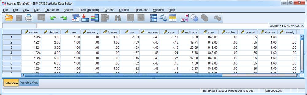
To illustrate, we will implement the syntax file for the High School and Beyond example used in the textbook by Raudenbush and Bryk (2002) and which figures in software tutorials by Peugh and Enders (2005) and Singer (1998). In this example, there are 7185 students nested within 160 high schools. Within SPSS, the data looks like this:

The model considered here evaluates the within-school effect of socioeconomic status on math achievement and whether this effect varies over schools. In equation form, the model is

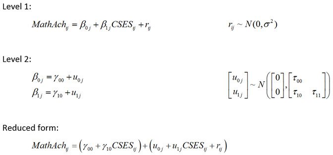
Note that the level-1 units are students within schools, the level-2 units are schools, i indexes the student, j indexes the school, MathAch is student math achievement, and CSES is a within-school centered measure of the student's socioeconomic status. The level-1 residuals are denoted r with variance sigma-squared, and the Level-2 random effects are denoted with u's and their variances and covariances are represented by tau's.

To fit this model in SPSS, we would use the following syntax (see Peugh and Enders, 2005, for a detailed explanation of these commands):

MIXED mathach WITH cses
/FIXED=cses
/RANDOM=INTERCEPT cses | SUBJECT(school) COVTYPE(UN)
/PRINT=SOLUTION TESTCOV G
/SAVE=FIXPRED.

The last line saves out predicted values for MathAch based solely on the fixed-effects portion of the model. These predicted values will be added to our data set with the default variable name FXPRED_1 and will be used when we compute the random effect estimates. Of course, we could also fit the model and save these predicted values via point-and-click pull-down menus.

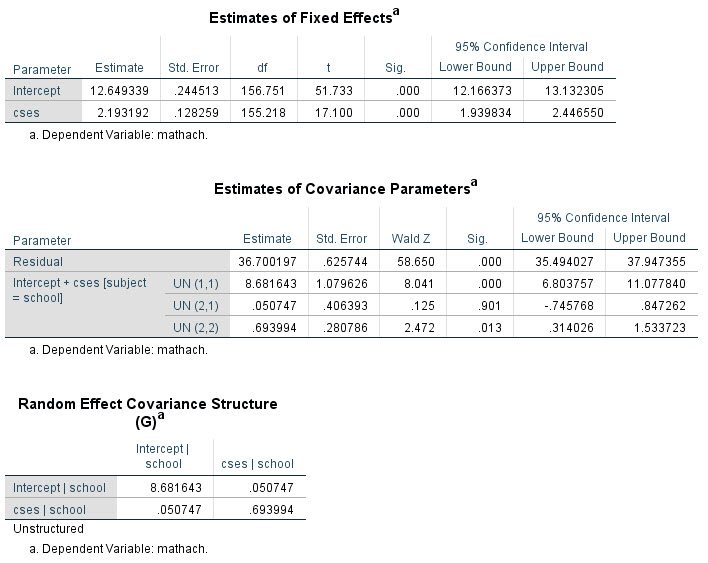
The relevant output from this model is shown here:

Now we can compute the empirical Bayes' estimates of the random effects from the appropriate equations. First, note that this syntax should be run only with the specific sample on which the analysis was based -- observations with missing values on the model outcome or predictors should therefore be removed before proceeding (since these observations would have been excluded from the analysis). Second, if the data are not already sorted on the Level 2 unit ID variable, it's a good idea to do this before proceeding:

SORT CASES BY School(A).

Next, because we are going to compute unique random effect estimates for each Level 2 unit (school), we need to designate that we will be looping through all 160 schools here:

*set MXLOOP to # Level 2 units.
SET MXLOOP = 160.

Now, we go into the SPSS MATRIX command and compute the estimates, beginning with the following lines of code (*'s indicate comments rather than syntax):

MATRIX.
*Input # Level 2 units.
COMPUTE N = 160.
*Input estimated covariance matrix for Level 2 random effects (Tau, referred to as G by SPSS).
COMPUTE Tau = {8.681643, .050747;.050747, .693994}.
*Input estimated residual variance at Level 1 (Sigma2).
COMPUTE Sigma2 = {36.70020}.
*Indicate Level 2 ID variable.
GET ID / VARIABLES school.
*Indicate dependent variable.
GET y / VARIABLES mathach.
*Indicate variable name for predicted values based on fixed effects, obtained with FIXPRED option of SAVE subcommand.
GET fixpred / VARIABLES FXPRED_1.
*assign labels for ID variable and random effects.
COMPUTE labels = {"school", "u0", "u1"}.

The user must enter the appropriate values for the variables and estimates referenced in these lines, with things that may need changing indicated in bold font. For instance, in the line COMPUTE Tau = { }, we input the random effect variance and covariance estimates as reported to us in the SPSS output for the G-matrix (elements separated by commas, rows separated by semi-colons). Likewise, in the line GET ID / VARIABLES school, we input "school" because this is the ID variable for the level-2 units in this analysis.

Next, if the model includes only a random intercept this line is included (otherwise comment it out):

COMPUTE Z= MAKE(NROW(y),1,1).

Otherwise, if the model includes random slopes these lines are included (otherwise comment them out), with the first line modified to include the names of any predictors with random slopes (in this case, CSES):

GET Zpred / VARIABLES cses.
COMPUTE Zconst = MAKE(NROW(y),1,1).
COMPUTE Z = {Zconst, Zpred}.

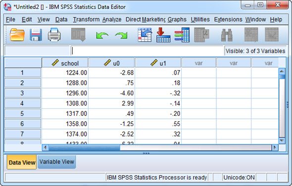
The rest of the syntax (not shown) runs without need for further modification. Running the full syntax generates a data file that includes the indicated Level-2 ID variable as well as the random effect estimates (here called u0 for the intercept and u1 for the CSES slope), as shown here:

These random effect estimates are now available for further use, such as to conduct model diagnostics or generate plots. Note that we cross-checked the syntax by comparing these values to those produced internally using the MIXED procedure of SAS and the random effect estimates were identical.

Important Notes

A few things to keep in mind when using this code...

• • For some reason that is not clear to us, SPSS generates an error message whenever the syntax is run: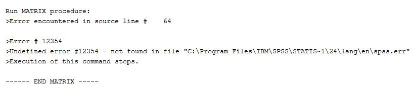This error, however, appears to be of no consequence. It does not stop the syntax from running and the random effect estimates produced by the syntax match those generated by other software programs.
  • There are alternative ways that this procedure could be streamlined and automated, but we present the above code to highlight precisely how these estimates are computed and obtained. The syntax could be simplified by making use of the Output Management System (OMS) of SPSS to read out the relevant estimates from the MIXED command and by putting the syntax into an SPSS macro.

References

Peugh, J.L. & Enders, C.K. (2005). Using the SPSS MIXED procedure to fit cross-sectional and longitudinal multilevel models. Educational and Psychological Measurement, 65, , 717-741.

Raudenbush, S. W., & Bryk, A. S. (2002). Hierarchical linear models: Applications and data analysis methods (2nd ed.). Newbury Park, CA: Sage.

Singer, J. D. (1998). Using SAS PROC MIXED to fit multilevel models, hierarchical models, and individual growth models. Journal of Educational and Behavioral Statistics, 24, 323-355